Euro 2020 Player Stats
Like most grad students, I suffer from intense guilt when doing anything “non-productive”. The guilt is directly proportional to the amount of hours spent on the non-productive activity. So, as you can imagine, watching every single game of Euro 2020 has been a turbulent ride.
As a Brit living in the US, I’ve been struck by how much Americans love to quantify things. This is particularly evident when it comes to sports, hence this tweet I wrote:
🇺🇸 American soccer commentators:
— Sophie Hill (@sophie_e_hill) June 13, 2021
“let me tell you how many assists this player got in the 2018-19 season”
🏴 English football commentators:
“the thing about this guy is, well, he’s got that extra bit of ~quality~ hasn’t he”
So, naturally, I thought I might allay some of my Euros-induced guilt by doing a bit of Euros data analysis! The UEFA website has all kinds of fascinating stats on players and teams. Here’s what they have for England captain Harry Kane:
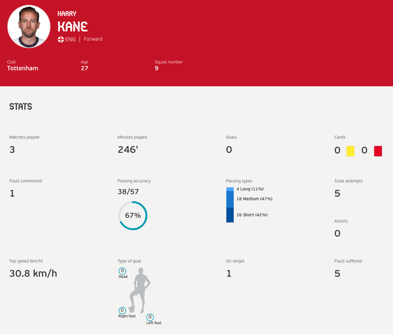
Stats for Harry Kane, from the UEFA website
BUT: annoyingly, it doesn’t seem possible to compare players across all these metrics. They have a page of “performance rankings” but those are based on a “specially devised algorithm” developed by sponsor FedEx (?).
And look, no disrespect to FedEx, but I’m not particularly interested in this arbitrary points system. I want to see all the underlying metrics.
So I inspect the source code of the player stats page, hoping that it’s being loaded from a hidden but easily-accessible database. Alas, there’s a hideous amount of Javascript. I can see an API key in there but after fiddling around with it for a few minutes I’m not able to access it.
The remaining option, of course, is brute-force web-scraping. After all, the player stats are publicly available on each player’s page – I just need to go through each one and store the values. There are two annoying complications here:
Not all players have the same set of stats. OK this does kind of make sense. We probably don’t need to know how many punches Harry Kane has made, or how many goals Jordan Pickford has scored. That’s ok. We’ll just store all the available stats for each player, and when we bind them all together there will be some missing values.
The stats themselves are formatted in a rather fancy way, like the pass completion rate being stored as a label on a spinner-graph image. This is going to be a manual job, but luckily there aren’t too many stats with idiosyncratic formatting.
So to scrape all the stats, I’m going to use 2 nested loops. The first loop iterates over each team and finds all the player URLs for that team. The second (nested) loop, iterates over the player URLs and extracts all the available stats for that player.
Here’s the bare bones of the code (with the content of that 2nd loop omitted because it’s long and dull):
# Step 1: Find all team urls
# go to the "teams" page and save html
team_url <- "https://www.uefa.com/uefaeuro-2020/teams/"
html <- paste(readLines(team_url), collapse="\n")
# find all hyperlinks on the page
matched <- str_match_all(html, "<a href=\"(.*?)\"")
# manually select the hyperlinks for teams
team_urls <- matched[[1]][15:38,2]
team_urls <- paste0("https://www.uefa.com", team_urls)
# empty list to store output
final_output <- list()
# Step 2: Loop over the teams,
# to extract all player urls for each team
for (i in 1:length(team_urls)){
# save html and search for hyperlinks
html <- paste(readLines(team_urls[i]), collapse="\n")
matched <- str_match_all(html, "<a href=\"(.*?)\"")
# save hyperlinks that contain the word "players"
player_urls <- matched[[1]][str_which(matched[[1]][,2], "players"),2]
player_urls <- paste0("https://www.uefa.com", player_urls)
# replace special characters for Danish names!!
player_urls <- gsub("æ", "æ", player_urls)
# then encode in URL format
player_urls <- URLencode(player_urls)
output <- list()
# Step 3: Loop over the players for a given team,
# and extract player stats
for (j in 1:length(player_urls)){
# save html
player_html <- player_urls[j] %>% read_html()
## ...
# OMITTED: extract player stats and save output
## ...
output[[j]] <- my_dat
}
}
# Once all player info has been scraped for each team,
# combine into one dataframe and store in final_output list
temp <- do.call("bind_rows", output)
rownames(temp) <- NULL
final_output[[i]] <- temp
temp <- NULL
}To extract each player’s stats, I used the Chrome extension Selector Gadget to identify elements on the page. As you can see, the stats are stored in HTML div’s with the class statistics--list--data.
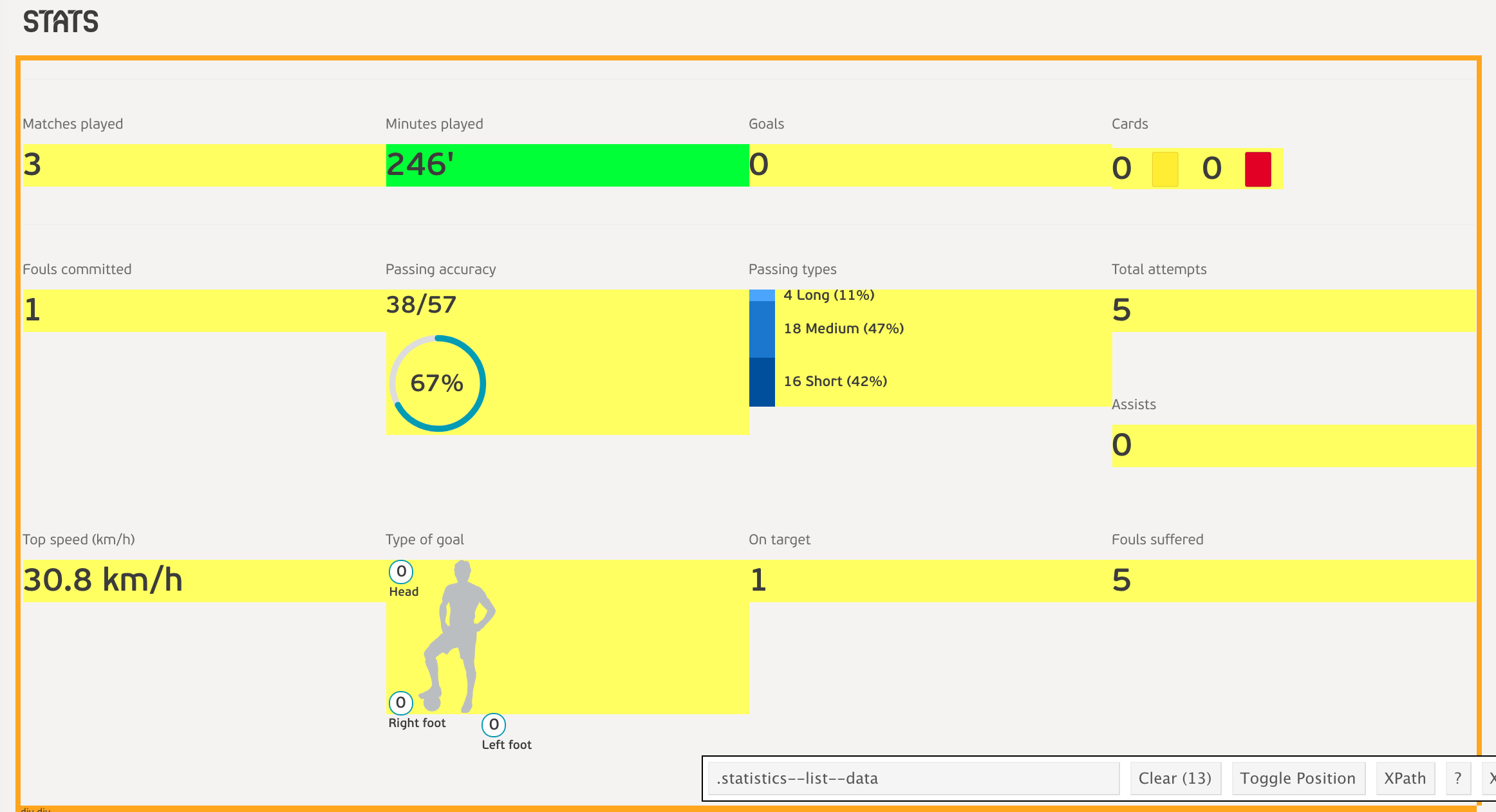
Identifying elements using Selector Gadget
As I said, a few of these have some funky formatting, so we can also use Selector Gadget to narrow in on one particular element and do some tidying up.
The eagle-eyed among you will notice that I had to do an extra bit of cleaning on the player URLs because some of the Danish players have special characters in their names and we need to convert them correctly into ASCII format for the URL. So, for example, Simon Kjær’s URL becomes:
https://www.uefa.com/uefaeuro-2020/teams/players/108509--simon-kj%C3%A6r/
Anyway, once those small quirks are ironed out, the code works! It is extremely inefficient, when you think about it, since it has to read a whole web page just to get one row of the data. But UEFA did not make it easy for me!
Here’s a snippet of the data:
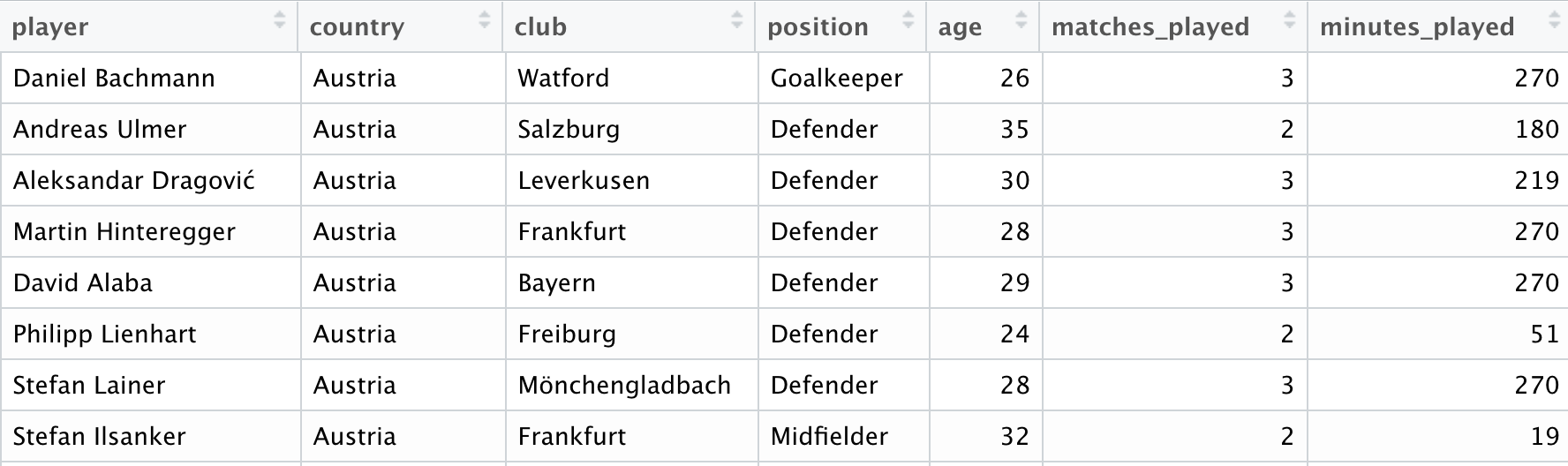
Snippet of the data
Now the next step is to turn this dataset into an interactive object that lets the user filter, sort, and select different variables. To do that, I’m going to use the DT R package, which is an R interface for the Javascript library Datatables.
I’m in a whimsical mood so I decided to add some emojis to the country names. We can do this with the R package emo, which will find and print an emoji based on a keyword. For most countries, we can find it right away. For others, we need to dig a bit further…
library(emo)
emo::ji_find("portugal")
## # A tibble: 1 x 2
## name emoji
## <chr> <chr>
## 1 portugal 🇵🇹emo::ji_find("czech_republic")## # A tibble: 1 x 2
## name emoji
## <chr> <chr>
## 1 czech_republic 🇨🇿emo::ji_find("turkey")## # A tibble: 2 x 2
## name emoji
## <chr> <chr>
## 1 turkey 🦃
## 2 tr 🇹🇷Another quirk that stumped me for several hours is that the function emo::ji doesn’t appear to be vectorized, so we need to use purrr::map_chr to apply it over a vector of country names:
dat <- dat %>% mutate(country_emoji_text =
                        case_when(country=="North Macedonia" ~ "macedonia",
                                  country=="Turkey" ~ "tr",
                                  TRUE ~ tolower(gsub(" ", "_", country))))

dat$country_emoji <- map_chr(dat$country_emoji_text, emo::ji)
dat$country2 <- paste0(dat$country, " ", dat$country_emoji)
OK, back to the task at hand. How do we turn this dataset into an interactive datatable?
d <- datatable(datx,
               # Set readable column names
               colnames = c("Player" = "player",
                            "Country" = "country2",
                            "Club" = "club",
                            "Position" = "position",
                            "Age" = "age",
                            "Goals" = "goals",
                            "Assists" = "assists",
                            "Attempts" = "total_attempts",
                            "Attempts on target" = "on_target",
                            "Distance covered" = "distance_covered_km",
                            "Top speed" = "top_speed_km_h",
                            "Total passes" = "passes_total",
                            "Pass completion" = "pass_accuracy",
                            "Tackles" = "tackles",
                            "Blocks" = "blocks",
                            "Balls recovered" = "balls_recovered",
                            "Clearances" = "clearances_completed",
                            "Fouls committed" = "fouls_committed",
                            "Fouls suffered" = "fouls_suffered"),
               # apply some basic styling to the table
          class = 'hover compact stripe',
          # a custom Javascript function to make sure the
          # row numbers are dynamically updated
          callback=JS("table.on( 'order.dt search.dt', function () {
                                table.column(0, {search:'applied', order:'applied'}).nodes().each( function (cell, i) {
                                      cell.innerHTML = i+1;});}).draw();"),
          extensions = c('Buttons',
                         'Scroller',
                         'Select', 'SearchPanes'),
          options = list(dom = 'Btip',
                         pageLength = 30,
                         buttons = list(list(extend = "colvis",
                                             columns = c(6:19),
                                             text="Select stats"),
                                        list(
                                          extend = "searchPanes",
                                          config = list(
                                            dtOpts = list(
                                              paging = FALSE
                                            )))),
                         deferRender = TRUE,
                         #scrollY = "450px",
                         scrollX = TRUE,
                         scrollCollapse = TRUE,
                         paging = TRUE,
                         language = list(searchPanes = list(collapse = "Filter"),
                                         colvis = list(collapse = "test")),
                         columnDefs = list(
                           list(width = "15px", targets=c(0,5)),
                           list(width = "200px", targets=c(1)),
                           list(width = "100px", targets=c(2:4)),
                           list(width = "15px", targets=c(7:19)),
                           list(visible = FALSE, targets=c(7:9,10:11,14:19)),
                           list(searchPanes = list(show = FALSE), targets = c(1,5:19)),
                           list(searchPanes = list(show = TRUE, controls=TRUE), targets = c(2,3,4))
                         ))) %>%
  DT::formatString(columns=c(10), suffix="km") %>%
  DT::formatString(columns=c(11), suffix="km/h") %>%
  DT::formatString(columns=c(13), suffix="%")
Phew. That’s a lot. The DT package is great but it is very clear that we are writing R code to be transformed into Javascript. Hence the lists of lists of lists… Still, it’s great to have all that flexibility.
Now in general I would always prefer a graph over a table. However, if we want to compare LOTS of different observations (there are 470 players in the tournament!) on LOTS of different metrics, then a table is definitely the way to go.
Fortunately, we can build some of the visual heuristics of a graph into our table by using “databars”: basically a bar in each cell that corresponds to the magnitude of the cell’s value.
But in order to implement this, we going to need – yes, you guessed it – another loop! Why? Because if we tell datatable to create databars for all the numeric columns, the bars will be scaled by the minimum and maximum values across all those columns. This doesn’t make much sense, because we want to compare the relative magnitudes within a column. And, since our dataset includes things like goals and minutes played, we know that the range is going to vary greatly by column!
So here’s the loop:
# save list of colors
colors <- colorRampPalette(brewer.pal(min(sum(num),9), "Pastel1"))(14)

# iterate over columns 6 through 19
# (these are the numeric columns)
for (i in 6:19){
    d <- d %>%
      formatStyle(c(i),
                  # define the range and color for each column
                  background = styleColorBar(range(datx[,i], na.rm=TRUE), colors[i-5]),
                  backgroundSize = '98% 88%',
                  backgroundRepeat = 'no-repeat',
                  backgroundPosition = 'center')
    }
This loop generates these lovely, column-specific databars!
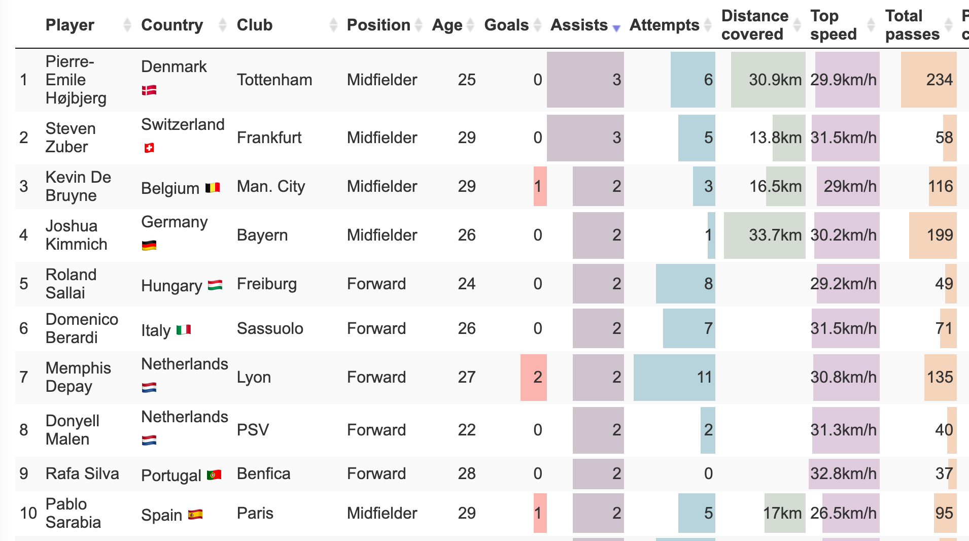
Table with colored databars indicating cell values
The only other piece of code I used here was an inelegant way to add a bit of HTML at the top and bottom of the widget. At the top, I’m going to load my own custom CSS file (to specify the font, since otherwise it will vary from browser-to-browser) and add a large title. At the bottom, I’ll add a footer indicating the source of the data. Finally we just need to save the table as a standalone HTML widget!
temp <- d %>% htmlwidgets::prependContent(
  htmltools::tags$head(list(
    htmltools::tags$link(href = "custom_css.css", rel = "stylesheet")
  ))
)

temp <- temp %>% htmlwidgets::prependContent(
  HTML(
    "<body><h1 style = 'font-family: Helvetica;'>EURO 2020 Player Stats</h1></body>"
  ))

temp <- temp %>% htmlwidgets::appendContent(
  HTML(
    "<body><span style = 'font-family: Helvetica;'>Stats from <a href='https://www.uefa.com/uefaeuro-2020/teams/'>UEFA</a></span></body>"
  ))

saveWidget(temp,"euro-2020-stats.html")
I uploaded this static file to my website, and so you can view the table and mess about with it to your heart’s content here!